![]()
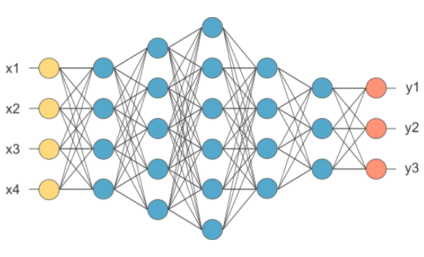
Our first fully connected neural network in TensorFlow/Keras
This example notebook provides a small example how to implement and train a fully connected neural network via TensoFlow/Keras on the MNIST handwritten digits dataset.
In [1]:
%tensorflow_version 2.x
In [2]:
import numpy as np
import matplotlib.pyplot as plt

from tensorflow import keras

%matplotlib inline
Load MNIST data, check its dimensions and let's look at a few random examples
In [3]:
(x_train, y_train), (x_test, y_test) = keras.datasets.mnist.load_data()
In [4]:
x_train.shape, y_train.shape, x_test.shape, y_test.shape
Out[4]:
In [5]:
def show_train_imgs(n=8, m=5):
    for i in range(m):
        for j in range(n):
            idx = np.random.randint(len(y_train))
            plt.subplot(int('1' + str(n) + str(j+1)))
            plt.imshow(x_train[idx], cmap='gray')
            plt.title(y_train[idx], fontsize=30)
            plt.axis('off')
        plt.show()
In [6]:
plt.rcParams['figure.figsize'] = (15, 5)
show_train_imgs(8)


In [7]:
x_train.min(), x_train.max()
Out[7]:
Normalize data & reshape to a 1D array instead of 2D matrix.
In [8]:
x_train = x_train.reshape(60000, 28*28)/255
x_test = x_test.reshape(10000, 28*28)/255

x_train.shape, x_test.shape, x_train.min(), x_train.max()
Out[8]:
In [9]:
y_train[:5]
Out[9]:
Conversion of the labels to one-hot encoded labels
In [10]:
y_train_oh = keras.utils.to_categorical(y_train)
y_test_oh = keras.utils.to_categorical(y_test)
y_train_oh[:5]
Out[10]:
We will use the so called Sequential API.
This API let's us to build neural networks with the following limitation: each layer's input is the output of the previous layer to build more flexible neural networks we will use the Functional API
The Sequential API...
- builds up layer-by-layer
- you can pass activation functions as an argument to most of the layers
- or you can create activation layer
- .summary()
- model needs to be compiled before training
- you need to set the loss function
- optimizer
- metrics
- any callbacks (functions to run after/before epochs, batches, etc)
- after compiling you may train your model
- #epochs
- batch size
- train data
- validation data can be provided
- you can also generate predictions with a trained model
In [11]:
model = keras.Sequential()
model.add(keras.layers.Dense(784, activation='relu', input_dim=784))
model.add(keras.layers.Dense(512, activation='relu'))
model.add(keras.layers.Dense(256, activation='relu'))
model.add(keras.layers.Dense(128, activation='relu'))
model.add(keras.layers.Dense(10, activation='softmax'))
In [12]:
model.summary()
In [13]:
784*784+784, 784*512+512, 512*256+256, 256*128+128, 128*10+10
Out[13]:
In [14]:
model.compile(loss='categorical_crossentropy', optimizer=keras.optimizers.SGD(lr=1e-2), metrics=['accuracy'])
With GPU 1 epoch ~3s.
If you feel your model is much slower activate GPU on Google Colab via Runtime $\to$ Change runtime type $\to$ Hardware acceleraton $\to$ GPU During training the most importrant summary is shown. You can also save trianing history.
In [15]:
history = model.fit(x=x_train, y=y_train_oh, batch_size=64, epochs=15, validation_data=(x_test, y_test_oh))
In [16]:
plt.plot(history.history['loss'], label='train loss')
plt.plot(history.history['val_loss'], label='val loss')
plt.xlabel('epochs', fontsize=15)
plt.legend(fontsize=20)
plt.show()
plt.plot(history.history['accuracy'], label='train accuracy')
plt.plot(history.history['val_accuracy'], label='val accuracy')
plt.xlabel('epochs', fontsize=15)
plt.legend(fontsize=20)
plt.show()


>97%, not too bad, but why not 100%?
Let's check the predictions, where the model goes wrong. Errorneous predictions are highlighted with a red dot. Also, from the learning curves above we can see, that the model is still not fully trained, the results are still improving.
In [17]:
def show_predictions(n=5, m=5):
    for j in range(m):
        idx_start = np.random.randint(len(x_test) - n)
        preds = model.predict(x_test[idx_start:idx_start+5])
        true_labels = y_test[idx_start:idx_start+5]

        for i in range(n):
            plt.subplot(int('1' + str(n) + str(i+1)))
            predstr = 'pred: ' + str(preds[i].argmax()) + ', prob: ' + str(int(np.round(preds[i].max()*100,0))) + '%'
            plt.title(predstr + ' / true: ' + str(true_labels[i]),fontsize=10)
            plt.imshow(x_test[idx_start+i].reshape(28, 28)*255, cmap='gray')
            if(preds[i].argmax() != true_labels[i]):
                plt.scatter([14], [14], s=500, c='r')
            plt.axis('off')
        plt.show()
In [18]:
show_predictions(m=20)


